

Portfolio Project – Top 1000 movies on IMDb
For this portfolio project, I wanted to create an exploratory data analysis (EDA) on a dataset of the top 1000 movies on IMDb using Python in a Jupyter notebook. What makes this project especially interesting is the fact that it's an interactive report using Panel. Although you would have to download the Github repository to see for yourself since it lacks the capability to run interactive applications, below you will find the (static) highlights of the EDA. Below, you will find a shortened version of the EDA you will find in the aforementioned Github repo.
Note: images can be made larger when clicked on.
Introduction
Objective
Welcome to this exploratory data analysis (EDA). In this report we will dive into the world of cinema by analyzing a dataset on the top 1000 movies on the IMDb website. The objective of this EDA is twofold:
• to give a high level overview of the dataset itself,
• to uncover possible patterns, trends and outliers in the data.
Hopefully this might lead to useful insights and, possibly be a starting point for further exploration. To do so, various charts, plots and heatmaps have been employed to visualize key elements of the dataset, such as possible correlation within the dataset, distributions, outliers, etc.
Dataset
The dataset contains data on the best rated movies on the IMDb website, which is an online database on, among other things, movies and TV series. (IMDb stands for ‘Internet Movie Database’.) For many people, the IMDb website is their go-to resource to look up information on movies and casts. One of the central pillars of the popularity of IMDb is their IMDb rating system: a 10-star scale reflecting the collective opinion of the voters on movies and TV-shows. Every user is able to cast votes on movies on the IMDb website (one vote per movie), which are then aggregated and summarized as an IMDb rating. This dataset contains the top 1000 movies, mainly based on their respective IMDb rating.
Link to original Dataset: Kaggle.com
Framework
The framework for this interactive report has been developed and generously made available to others by Sunny Solanki through an MIT license. What makes this framework particularly interesting is the fact that it has been entirely written in Python. The obvious benefit is that this EDA is not reliant on software like Tableau, Power BI or Looker Studio.
Link to original framework: Github
Cleaning the Data
The quality of your insights is generally only as good as the quality of your data. It comes as no surprise that data cleaning is an essential step in an EDA. Here, we will explore the data cleaning process the top 1000 IMDb movies dataset has undergone. Despite the dataset’s relatively good initial condition, there were still adjustments necessary to ensure its integrity and usability. Below, you will see the schema of the dataset before the cleaning process on the left side and the schema after the cleaning on the right side. You will also see a short summary of the most important steps taken in the data cleaning process, which laid the foundation for the insights in the rest of this exploratory data analysis.
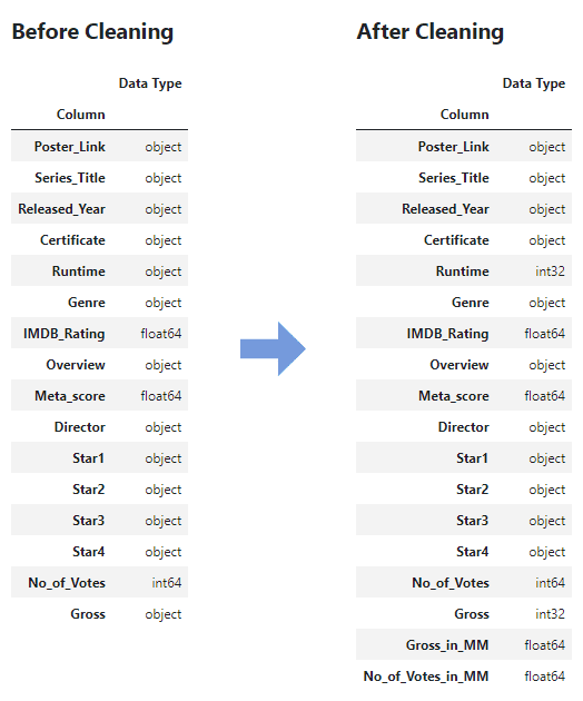
What cleaning has been done?
• The Released_Year column contained a non-numeric value, which needed to be replaced with the correct year of release.
• The Runtime column was of datatype 'object' and needed to be converted into an integer (int32) first.
• The Gross column was of datatype 'object' as well, and needed to be converted into an integer (int32).
◦ The values in this column were formatted like this: '28,341,469'. However, they were were treated like text (a.k.a. strings) rather than numbers. In order to convert them to numbers, the commas had to be removed so as to look like this: '28341468'. Only after could these values be converted into numbers.
• Seeing as the No_of_Votes column contains relatively large numbers, for the sake of readability I have added a column to the dataset called No_of_Votes_in_MM, in which I have divided the values by a million so as to get the values in millions. This makes labels on charts and plots far easier to read.
◦ Due to the division, the datatype of this new column automatically changed to a floating-point number (float64).
The same was done for the Gross column, for which I have created a new column called Gross_in_MM.
• The rest of the data transformations have been done separately for the specific charts and plots themselves.
Distribution of IMDb Ratings
The most important metric in the entire dataset and on the IMDb website alike is the so called IMDb rating. The IMDb rating is a number ranging from 1 to 10, reflecting how much people like that particular movie, with 1 being worst and 10 being best. The IMDb rating is a weighted average per movie, primarily composed of user ratings. Given the importance of the IMDb ratings, we will take a look at how spread out they are in the dataset. This will give us an insight in what people tend to value in movies, while simultaneously looking at possible outliers.
Below you will see a boxplot; a chart that captures the essence of distribution with simplicity and precision. For those who are unfamiliar with reading boxplots: below the plot you will find an explanation, along with the most important takeaway as bulletpoints underneath. Finally, we will zoom in on the outliers the boxplot has revealed, among which you will most likely recognize at least a few movies.
How are the IMDb ratings distributed in our dataset?
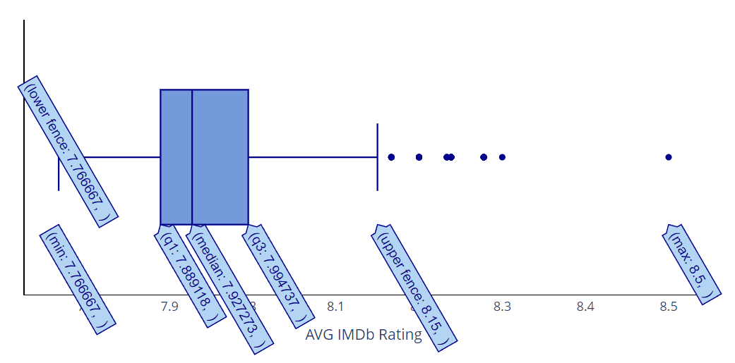
In the boxplot (a.k.a. a box and whisker plot) below we see the distribution of the IMDb ratings in this dataset. Since reading boxplots might not be intuitive for everyone, the actual EDA contains an extra description on how to read one. For the sake of brevity, this description is omitted from this shortened version.
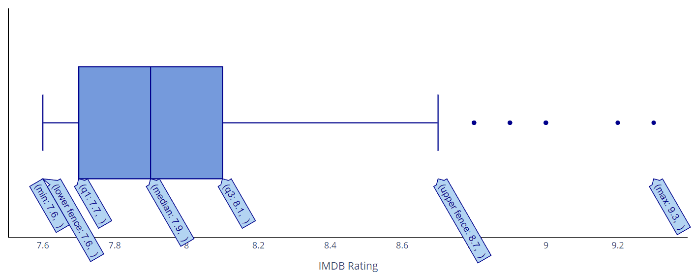
In our boxplot, the median is 7.9. This means that half of the IMDb ratings is equal to or below it (everything to the left of the median), and half of it is equal to it or above it (everything to the right of the median).
• The first observation we can make is that the ratings below the median are cramped in a much smaller space than the ratings above it. This implies that the distribution of the ratings equal to or below the mean are much more concentrated than the ones equal to or above it.
• We can also see that the distribution around the median is symmetrical, because the median is in the middle of the box, equidistant from the left (Q1) and right (Q3) side of the box. This symmetry implies that the IMDb ratings are uniformly distributed across this part of the data, and suggests that the IMDb rating system is reliable and stable.
Q1 has a value of 7.7, the median sits at 7.9, and Q3 at 8.1
• This means that 25% of the movies have an IMDb rating of 7.7 or below, 50% of the movies have a rating of 7.9 or below, and 75% of the movies have a rating of 8.1 or below.
• This also means that 50% of the movies in our dataset have an IMDb rating between 7.7 and 8.1. Even by looking at the box itself, we can see that it's not very wide relative to the rest of the plot. This suggests that there is tight clustering around the median, which means that a lot of movies have an IMDb rating close to 7.9.
The left and right whiskers of a boxplot generally extend to (respectively) the lowest value within 1.5 * IQR of Q1, and the highest value within 1.5 * IQR of Q3.
• In our boxplot, the left whisker doesn't extend all the way to 1.5 * IQR of Q1. It should extend all the way to 7.7 - (1.5 * (8.1 - 7.7)) = 7.1, but instead it stops at 7.6. The reason for this is that the lowest value in our dataset is 7.6, so the left whisker cannot extend past it.
• This makes sense, because our dataset contains data on the top 1000 movies on IMDb, which means that there's a cutoff with the lower IMDb ratings not being part of the dataset.
• Seeing as the whisker to the left is shorter than the one on the right, it suggests that the data is skewed towards higher IMDb ratings. This means that the IMDb ratings of the right whisker (the higher IMDb ratings) are more spread out compared to those of the left whisker (the lower IMDb ratings), which are more concentrated or clustered together.
The dots on the right side of the plot represent outliers, which are data points which differ significantly from the rest, so much so that they fall outside the range (represented by the whiskers).
• All of the outliers are positioned on the right side of the plot, and none of them on the left side. This implies that all of the outliers have an exceptionally higher IMDb rating compared to the rest of the ratings. This makes sense, as outliers positioned on the left side of the plot would have to have exceptionally lower IMDb ratings, which in turn would have excluded them from the dataset altogether.
• Although only 5 outliers are visible on the boxplot above, it doesn't mean that there are only 5 movies with these IMDb ratings. Every dot represents a distinct IMDb rating rather than a single movie. In actuality, there are 13 movies spread out over these 5 dots, which are shown below:
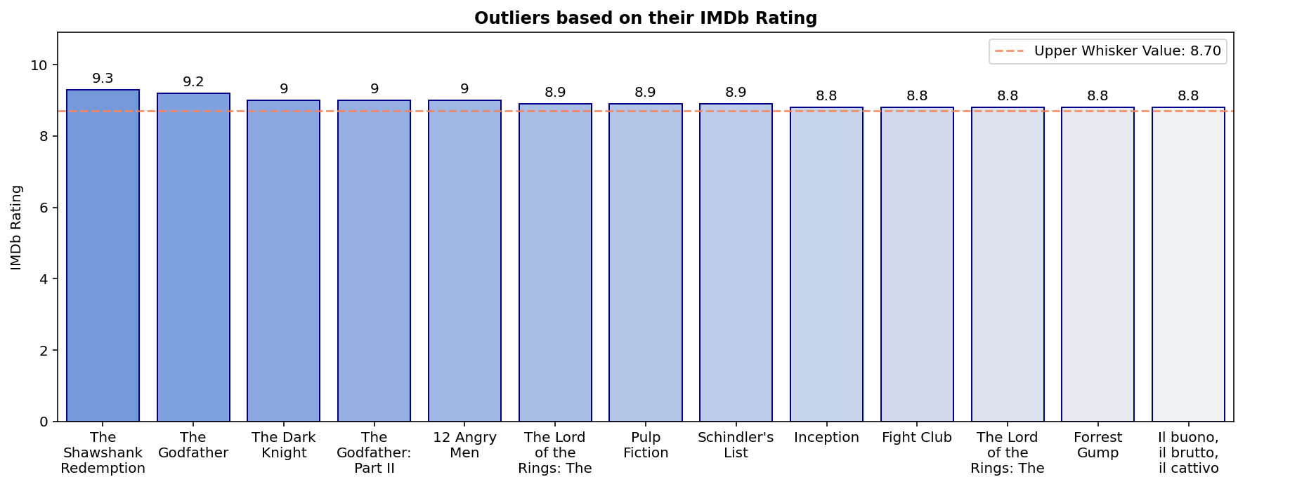
All of the movies on the bar chart above are outliers based on their respective IMDb ratings. On the boxplot we saw earlier, two whiskers were visible, depicting the range of the data. Everything exceeding this range was considered an outlier. Looking at the bar chart above, we also see a horizontal dashed line. This line represents the right whisker, so it lets us see by what margin the movies above have exceeded the range.
• When we look at the movie titles, most of us will recognize at least a couple of them. These movies being outliers can be explained by the fact that they are some of the most iconic movies in movie history.
• Most outliers seem to have barely exceeded the dashed line. However, the first two movies, The Shawshank Redemption and The Godfather, have done so ba relatively large margin. These movies embody such an impressive combination of artistic merit, viewer popularity and enduring legacy as influential works of cinema art, they have been rewarded with exceptionally high IMDb ratings.
IMDb Ratings over Time
To uncover more insights on IMDb ratings, we will now segment them by release year. Firstly, we will take a look at a time series (the chart below) to gain perspective on how the average IMDb ratings of the movies in our dataset have changed over time. Then, we will zoom in on the outliers which were uncovered by the time series and visualize them using a boxplot, table and several bar charts.
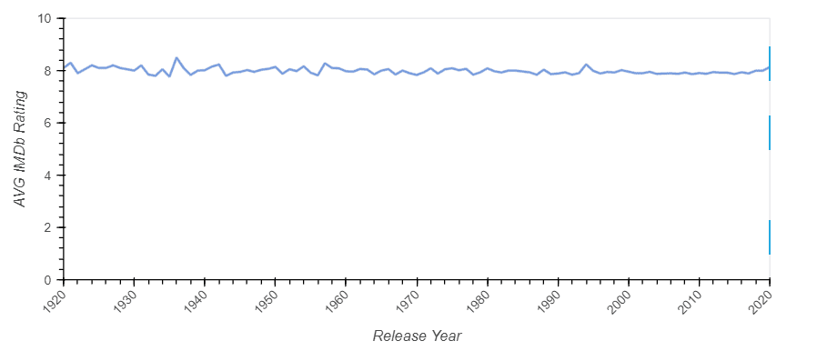
On first glance, looking at the average IMDb rating per year on the time series above, we can see that the line doesn't seem to have any major peaks or drops. It looks relatively steady, with an overall yearly average IMDb rating of 7.99, and lows and highs of respectively 7.77 and 8.5. However, if we look closely, we can certainly see a few peaks. If the values of these peaks are high enough, they will be considered outliers. In other words: a year is considered an outlier if it has an exceptionally higher (or lower) average IMDb score compared to the rest of the release years.
To get a clearer view of the outliers, let's look at the boxplot and accompanying table below. The boxplot shows us how the average IMDb ratings per release year are distributed. The dots on the right side of the boxplot are the outliers. Since none of the dots are positioned on the left side, it means that all of the outliers are positive. In other words: all of them had an exceptionally higher score relative to the rest of the release years. This makes sense, because movies with exceptionally low IMDb scores wouldn't be included in this dataset in the first place.
| | Release Year | AVG IMDb Rating | Movie Count | Outlier |
|---|---|---|---|---|
| 1 | 1936 | 8.5 | 1 | positive |
| 2 | 1921 | 8.3 | 1 | positive |
| 3 | 1957 | 8.28 | 9 | positive |
| 4 | 1994 | 8.24 | 13 | positive |
| 5 | 1942 | 8.23 | 3 | positive |
| 6 | 1924 | 8.2 | 1 | positive |
| 7 | 1927 | 8.2 | 2 | positive |
| 8 | 1931 | 8.2 | 3 | positive |
| 9 | 1954 | 8.17 | 6 | positive |
• Although it can't clearly be seen in the boxplot due to multiple years having the same average IMDb rating, there are 9 outliers in total. When we look at the table to the right of the boxplot above, we see a list of all the outliers, sorted from the highest average IMDb rating (top) to the lowest (bottom).
• Out of all the outliers, the year 1936 has the highest average IMDb rating: an 8.5. This is especially visible on the boxplot, as it is the dot all the way to the right. Although this average seems exceptionally high, when we look at the Movie Count column in the table, we see that this can be explained by the fact that only 1 movie released in 1936 has made it into the dataset.
• When we glance at the other rows in this column, most of the outlier years seem to be based on a relatively low amount of movies as well, which can explain their outlier status.
• Out of all of the outlier years, only these years stand out based on their movie count: 1954, 1957 and 1994. To see what makes these years outliers, we have to take a closer look.
What makes the years 1954, 1957 and 1994 outliers
Above, we have seen that the years 1954, 1957 and 1994 stand out as outliers because they are based on more movie releases than the rest of the outlier years: 6, 9 and 13 movies, respectively. Below, we will take a look at what movies each separate outlier year is comprised of.
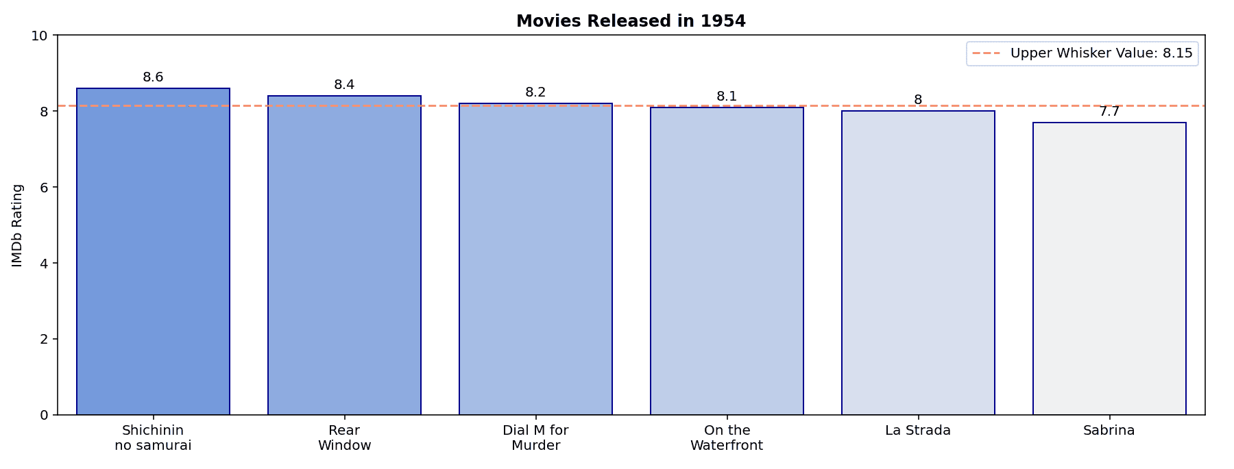
All of the movies released in the outlier year 1954 are shown in the bar chart above, with each bar being a separate movie. The height of the bars represents their respective IMDb ratings, with the highest rated movie positioned to the left and the lowest rated movie to the right. Similarly to the bar chart we saw before, we also have a dashed horizontal line. The value of this line, which in this case is 8.15, represents the value of the right whisker on the boxplot we saw earlier. This value marks the threshold of a value being an outlier. Since we are looking at outlier years, it means that the average IMDb rating of all the movies released in the particular year needs to exceed the value of the dashed line in order to be considered an outlier.
• Looking at the bar chart above, we see that half of the movies released in 1954 have an IMDb rating above the dashed line, and half of the movies have an IMDb rating lower than it.
• However, the two leftmost movies (Shichinin no samurai and Rear Window) are well above the dashed line, with ratings of 8.6 and 8.4 respectively, yet only one of the lower rated movies to the right (Sabrina) is well below the threshold, with an IMDb rating of 7.7.
• It seems that the IMDb ratings of the two leftmost movies are high enough to compensate for the movie on the right, which pulls the average IMDb rating for the year 1954 up to 8.17. Since this average exceeds the upper whisker value of 8.15, it makes the year 1954 an outlier.
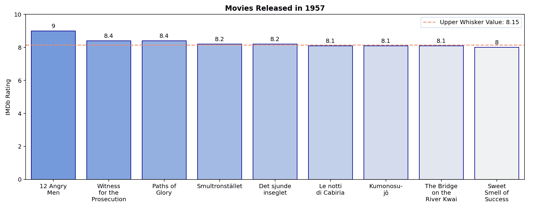
The bar chart above shows us all of the movies released in the year 1957, along with their respective IMDb ratings. The bar chart is sorted by IMDb rating, from the highest on the left to the lowest on the right. Similarly to the 1954 bar chart we saw earlier, we have a dashed, horizontal line denoting the value of the upper whisker (8.15), marking the threshold of a value being an outlier.
• Similar to the 1954 bar chart we saw before, the 1957 bar chart above shows that a little more than half of the movies have an IMDb rating exceeding the dashed line, while the other half falls below it.
• This time, however, the lower half dips below the dashed line only slightly, yet the upper half exceeds it with quite a margin. Especially the first movie, 12 Angry Men, with an IMDb rating of 9.0, rises above the dashed line quite a bit, pulling the total average IMDb rating for the year 1957 well above the upper whisker value to 8.28.
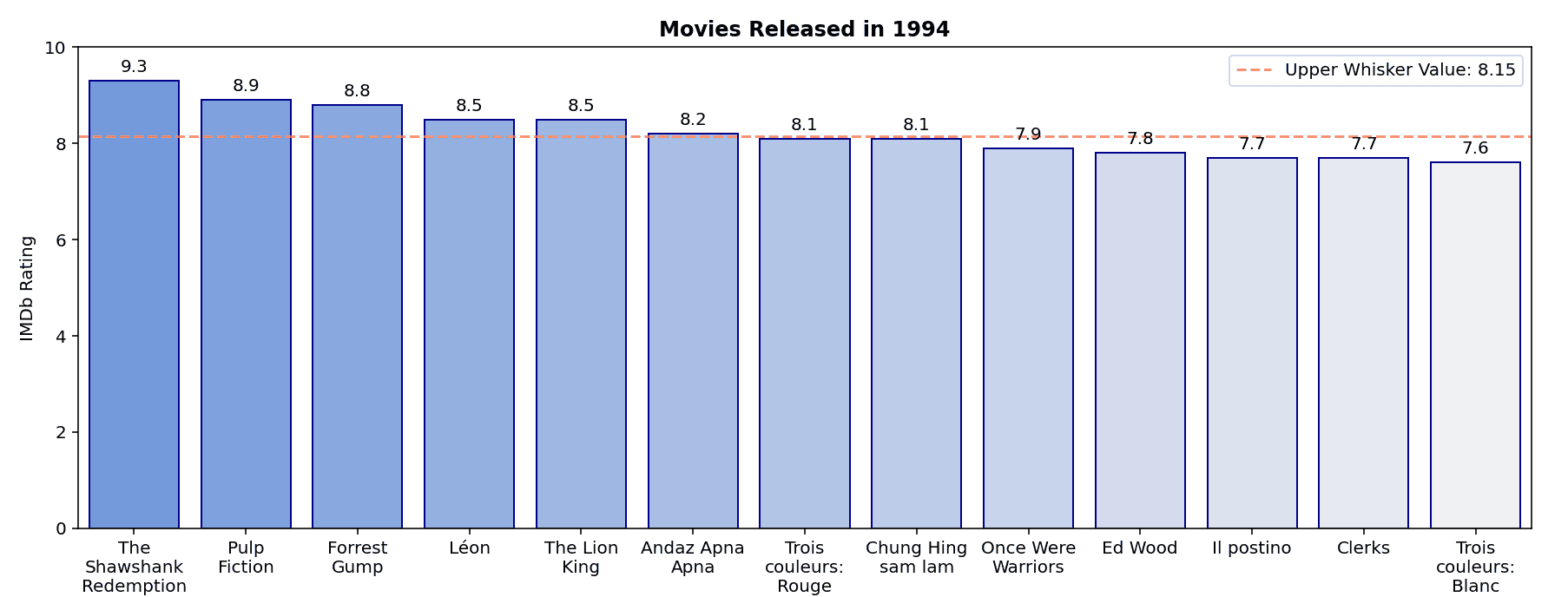
Out of all the outlier years 1994 tops the list when it comes to movie count, with a total of 13 movies released during this year. Out of these 13 movies, 6 of them exceed the upper whisker value of 8.15 (represented by the dashed line), and a little more than half of the movies fall below this threshold.
• It might be a bit hard to see on the bar chart above, but the movies which exceed the dashed line do so with a bigger margin compared to the negative margins of the movies which fall below it.
• To illustrate this in numbers:
◦ The median of the IMDb ratings for the year 1994 is 8.1, which means that half of the movies released in this year have IMDb ratings above it, and half of them score below it. Not a weak median value by any means, but it is still below the value of the dashed line.
◦ When we look at the average IMDb rating of all the movies above the dashed line, we get a value of 8.7. The movies below the dashed line have an average IMDb rating of 7.84. This suggests that the collective IMDb ratings of the upper half easily compensates for the collective IMDb ratings of the lower half of the movies.
• Looking at the bar chart, we can see that especially the first three movies, The Shawshank Redemption (the number 1 ranking movie in the entire dataset), Pulp Fiction and Forrest Gump, with respective IMDb ratings of 9.3, 8.9 and 8.8, pull the total average IMDb rating for 1994 up to 8.24, making it a relatively strong outlier.
Correlation
In this part of this exploratory data analysis, we take a look at the relationships between certain columns. This is done by using correlation, which is a statistical concept which helps us understand how two variables are related to each other. For example, if the values in one column go up, what tends to happen with the values in other columns? Do they go up, down or stay the same? By understanding such relationships, it helps us get a better understanding of the data and, in turn, can help us make better datadriven decisions. However, it is always important to keep in mind that correlation does not imply causation. In other words: just because two things are correlated doesn't mean that one causes the other.
We will first take a look at the heatmap below to check the correlation between the numeric columns in the dataset. The values in the heatmap are the correlation coefficients (sometimes expressed as the letter r) of those particular columns, which shows us how the two columns are related. The correlation coefficient has a standard minimum value of -1 and a maximum value of 1. The closer this value is to -1 or 1, the stronger the (negative or positive) correlation will be. In our heatmap, we're really only interested in values if they're either -0.30 or lower or 0.30 or higher, otherwise the correlation is too weak to be of interest.
Note: the heatmap and the scatterplots below have been corrected for missing values in the Gross and Meta Score columns.
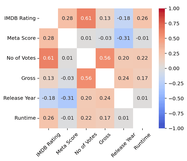
Correlation between columns in our dataset
On the heatmap above, three values have crossed the 0.30 or -0.30 thresholds: 0.61, 0.56 and -0.31. Below, we will first talk about the two positive values, after which we will shortly discuss the negative value. We will do so through the help of scatterplots. Scatterplots are visualizations which help us understand and interpret the relationship between variables. They enable us to do several things, like identify trends, determine correlation, spot outliers, visualize distribution, etc.
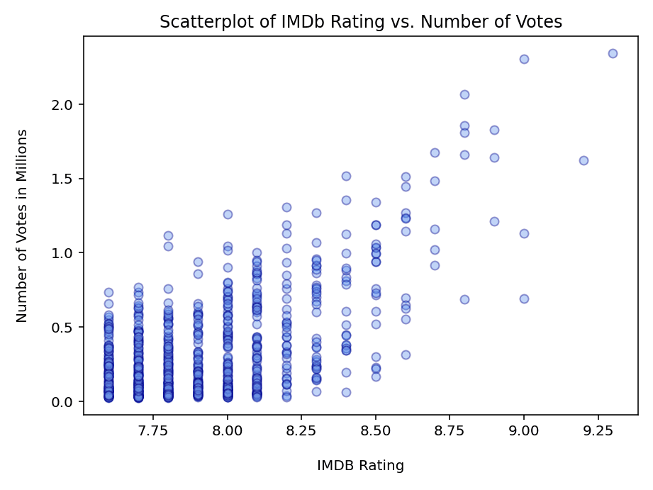
The first value, 0.61, is the correlation coefficient of the IMDB Rating column and the No of Votes column. Seeing as this value is higher than 0.30, it tells us there is a moderate positive correlation between the number of votes and the IMDb ratings. This suggests that movies with larger number of votes tend to have relatively higher IMDb ratings.
Looking at the scatterplot above, we see that it is a visualization of the same IMDB Rating and No of Votes columns, with IMDB Rating on the x-axis and No of Votes on the y-axis. Since every dot on this scatterplot is one movie rating, we can say that the higher its IMDb rating is, the farther the dot will be placed towards the right, and the more votes it has, the farther the dot will be placed towards the top of the plot. When we look at the scatterplot as a whole, the following is visible:
• Looking at how the dots are distributed on the plot, we can see the dots fan out from the bottom left corner towards the top right corner. This, paired with a correlation coefficient of 0.61, suggests that movies with higher IMDb ratings tend to have more votes.
• The colors of the scatterplot (which is unrelated to the color scale of the heatmap) show a darker blue in the bottom left corner of the plot, which is caused a by a large cluster of dots.
• A possible reason for this cluster could be the presence of indie-films or lesser-known movies in our dataset, which might not attract the same number of votes compared Hollywood blockbuster movies.
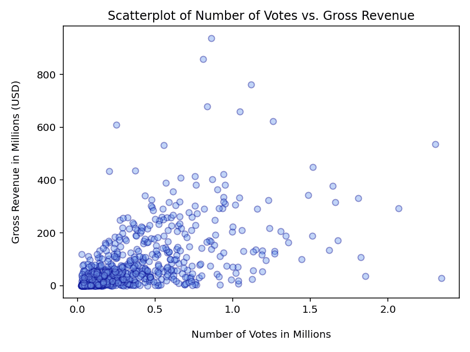
The second value which stood out from the rest was 0.56, which is the correlation coefficient of the Gross column and the No of Votes column. Looking at the scatterplot above, we see the No of Votes column on the x-axis and the Gross column on the y-axis. Looking at the scatterplot as a whole, we can say the following:
• Similar to the scatterplot to the first scatterplot, we see a cluster of dots in the bottom left corner, fanning out toward the top right. Paired with a correlation coefficient of 0.56, this suggests a moderate positive correlation between the No of Votes column and the Gross column. In other words: the gross revenue of movies tends to increase when the number of votes increases.
• This makes sense, as a relatively high gross revenue suggests a larger viewership. More people having seen the particular movie, in turn, could explain the higher number of votes.
• The high concentration of dots in the bottom left corner suggests that large amount of movies in our dataset tend to have relatively low amount of votes as well as a relatively low amount of revenue.
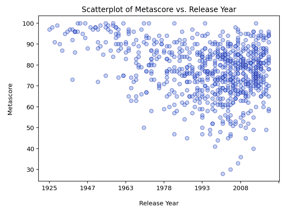
The final value which stood out from the rest is -0.31, which is the correlation coefficient of the Meta Score and Release Year columns. This is the only negative correlation coefficient in our heatmap which crossed the -0.30 threshold. Since it only barely did so, the negative correlation isn't very strong. In essence, a negative correlation between two columns means that when the values in one column go up, the values in the other column tend to go down. Looking at the scatterplot above, we see the Release Year column on the x-axis and the Meta Score column on the y-axis. As a whole, the scatterplot shows us the following:
• There is a large cluster of dots in the upper right corner. Since every single dot is one movie, this indicates that a large amount of movies have a release year of 1990-2020 and a Metascore of 60-95.
• When we move from left to right along the x-axis, we move on a timeline, from the past towards the present. When we look at how the dots are distributed on the scatterplot, we can see a downward trend, meaning that as we get closer to the present the Metascore seems to decrease.
• Obviously, there could be several explanations for it. E.g., perhaps critics have become more stringent over time, or maybe the criteria for a score have evolved. It might even be possible that critics tend to rate older movies more favorably due to their historical value or comparative quality.
Breakdown per Genre
Although IMDb ratings is perhaps the most important metric in the entire dataset, it's crucial to also segment the dataset in other ways. In this part we will break the dataset down by movie genre. Looking at the dataset through the lens of movie genres is a great way to uncover insights and identify patterns, as they reflect collective tastes and preferences of viewers. We will do this through the table below, where several other metrics are shown as well.
Given the fact that movies can be categorized as multiple categories at once, we will also take a look at which movie genres tend to be paired up and which pairs are unlikely.
| Genre | Movie Count | AVG IMDB Rating | AVG No of Votes | AVG Runtime in Mins |
|---|---|---|---|---|
| Drama | 724 | 8 | 240729 | 126 |
| Comedy | 233 | 7.9 | 225465 | 111 |
| Crime | 209 | 8 | 281322 | 123 |
| Adventure | 196 | 8 | 424952 | 125 |
| Action | 189 | 7.9 | 404172 | 126 |
| Thriller | 137 | 7.9 | 300050 | 119 |
| Romance | 125 | 7.9 | 200913 | 119 |
| Biography | 109 | 7.9 | 251898 | 135 |
| Mystery | 99 | 8 | 293463 | 121 |
| Animation | 82 | 7.9 | 268032 | 99 |
| Sci-Fi | 67 | 8 | 556242 | 120 |
| Fantasy | 66 | 7.9 | 347097 | 114 |
| History | 56 | 8 | 195434 | 143 |
| Family | 56 | 7.9 | 223472 | 114 |
| War | 51 | 8 | 194244 | 132 |
| Music | 35 | 7.9 | 139281 | 120 |
| Horror | 32 | 7.9 | 217860 | 102 |
| Western | 20 | 8 | 229475 | 134 |
| Film-Noir | 19 | 8 | 80185 | 100 |
| Sport | 19 | 7.9 | 256618 | 132 |
| Musical | 17 | 7.9 | 79613 | 140 |
In our IMDb movies dataset, movies are categorized by genre(s). In total, the dataset contains 1000 movies, belonging to 21 different genres. In the table to the left, you will see the dataset segmented by genre, with a count of the movies next to it, alongside certain other metrics.
With a total of 724 movies, the genre 'Drama' has the most movies ascribed to it by a relatively large margin. Interestingly, the average gross revenue for Drama isn't the highest by any means. When corrected for missing values in the Gross column, with an average of USD 46.06 million per movie, the genre Drama ranks only 13th (out of 21) for highest average gross revenue. This begs the question: if the category Drama is far from being the genre with the highest average gross revenue, why is it the category with the most movies ascribed to it in this dataset?
A possible (partial) explanation for this can be found in the fact that every single movie can be categorized as multiple genres at the same time. For instance, the movie 'The Dark Knight' is categorized as 'Action', 'Crime' and 'Drama'. It turns out that out of 724 movies belonging to the genre Drama, only 85 movies belong to this genre without simultaneously belonging to one or more other genres. This means that 639 movies are categorized as one or more other genres aside from being categorized as Drama. This could, in part, explain the relatively large amount of movies belonging to the genre Drama, but a deeper dive into the data is needed. Other genres containing movies ascribed to only that particular category are:
• Comedy with 13 movies,
• Western with 4 movies,
• Horror with 2 movies,
• Thriller with 1 movie.
Seeing as most movies are categorized as more than one genre, this raises the question about which movie genres tend to appear together, and which genres don't. To answer this question we will dive into genre pairings below.
Which movie genre pairings are most and least likely?
Determining which movie genres tend to occur together in our dataset and which don't is best done through a matrix. Below you will find a heatmap in which all movie genres with a correlation coefficient above 0.30 or below -0.30 have been included in a matrix. Since we now have some experience in reading such a heatmap after having read the one in the 'Correlation' section, reading this heatmap shouldn't be a problem.
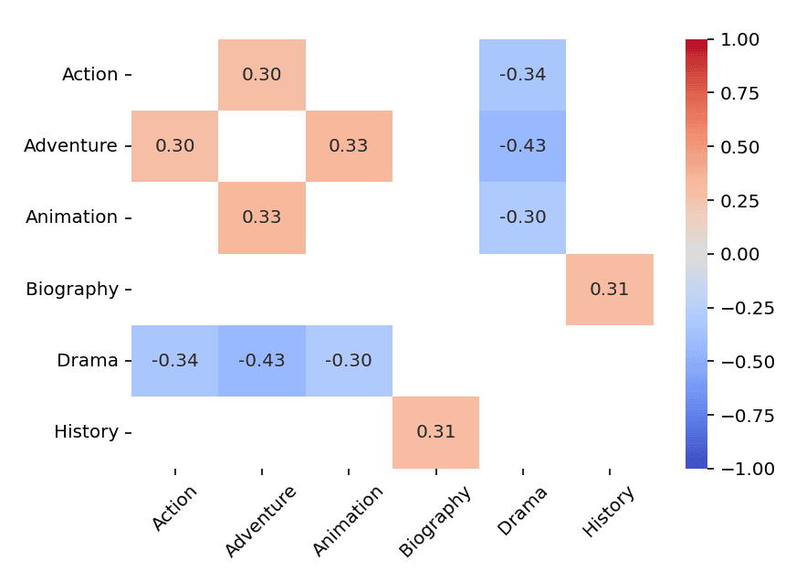
| | Genre Pairing | Correlation | Movie Count | AVG IMDb Rating | AVG No of Votes |
|---|---|---|---|---|---|
| 1 | Adventure - Animation | 0.33 | 52 | 7.9 | 346771 |
| 2 | Biography - History | 0.31 | 28 | 8 | 243191 |
| 3 | Action - Adventure | 0.3 | 83 | 8 | 558311 |
| 4 | Animation - Drama | -0.3 | 22 | 8 | 125985 |
| 5 | Action - Drama | -0.34 | 77 | 8 | 336382 |
| 6 | Adventure - Drama | -0.43 | 65 | 8 | 345658 |
As we can see on the heatmap above, the most likely genre pairings intuitively make sense.
• Adventure - Animation: animated movies are commonly adventurous. Since they aren't constrained by the bounds of reality, they allow creators to create new worlds full of adventure.
• Biography - History: biographies tend to be done on important historical figures; people who have had historical impact, shaping the course of history and society.
• Action - Adventure: adventurous movies are often action-packed, as it makes the adventure exciting. Adventure typically involves danger, and action-packed scenes highlights the bravery of the adventurer.
Conversely, the least likely paired genres also intuitively make sense, as they have an almost contrasting feel to them.
• Animation - Drama: adventure movies tend to have a more 'lighthearted' feel to it, while the genre drama seems more 'serious' in nature.
• Action - Drama: drama movies, which tend to have a more 'slow' feel to them, seem to form somewhat of a contrast to high-energy action movies.
• Adventure - Drama: drama also seems to conflict with animation as a genre, as the latter is generally used more often to portray something less serious.
What could contribute to the likelihood of certain genre pairings over others? Although it might not be a direct cause for a high correlation, an obvious thought would be money. Financial success can be a great indicator for market appeal. Although our dataset contains very limited financial data, it's still worth incorporating it in our visualizations. To do so, however, we will have to correct the data for missing values in the 'Gross' column. Below you will find a similar heatmap to the one above, but this time corrected for missing values. In the table below it, you will see additional data laid out in a table, including the average gross revenue per genre pairing.

| | Genre Pairing | Correlation | Movie Count | AVG IMDb Rating | AVG No of Votes | AVG Gross in MM |
|---|---|---|---|---|---|---|
| 1 | Action - Adventure | 0.34 | 76 | 8 | 603797 | 226.84 |
| 2 | Adventure - Animation | 0.32 | 43 | 8 | 401406 | 178.36 |
| 3 | Biography - History | 0.31 | 23 | 8 | 286452 | 55.33 |
| 4 | Animation - Drama | -0.35 | 13 | 7.9 | 145129 | 40.65 |
| 5 | Action - Drama | -0.36 | 59 | 8 | 421136 | 92 |
| 6 | Adventure - Drama | -0.47 | 52 | 8 | 413466 | 104.08 |
Similar to the previous table, the table above is sorted based on how likely a movie genre pairing is, with the most likely pairing on top (highest r) and the least likely pairing on the bottom (lowest r).
• Looking at the table above, it seems that the least likely genre pairing, Adventure - Drama, is not the pairing with the lowest average gross revenue. It actually has a higher average gross revenue than most of the more likely genre pairings above it.
◦ This suggests that financial outcome isn't the only factor to dictate likelihood of a genre pairing. One can image that it is a complex interplay of many factors, like artistic preferences, audience tastes and financial incentives.
• Another interesting observation (in both the first and second table) is that the movie count of the two genre pairings at the bottom is higher than some of the other genre pairings above them.
◦ For example, in the bottom table, when we compare the genre pairings Adventure - Animation (2nd place) with Adventure - Drama (6th place), the former pairing has a lower movie count (43 vs. 52) but is more likely to happen than the latter pairing (r = 0.32 vs. r = -0.47).
◦ The reason for this is that the likeliness of two movie genres being paired doesn't equate movie count. It's possible to have a high correlation with a low movie count, and conversely, a low correlation with a high movie count.
◦ In our example, the pairing Adventure - Animation is less common (movie count of 43) compared to the pairing Adventure - Drama (movie count of 52), but when the pairing does happen, it happens more consistently than the Adventure - Drama pairing.
What are the highest rated movies?
IMDb has become such a staple in the world of cinema that for many people it has become a trusted source in deciding whether or not watching a certain movie is worth their time. At the moment of writing (May 2024), IMDb.com has been the 44th most visited website on the internet in March 2024, according to Semrush. Such popularity comes with great power. A great quote to illustrate this is what the Financial Times had to say about IMDb:
"IMDb is one of the world’s most popular websites and functions as Hollywood’s memory. And that means IMDb has great power." – The Financial Times
The importance of IMDb ratings, therefore, shouldn't be understated. They not only reflect the opinions of large numbers of users, they might even influence movies' perception and success. This is why it's important to also have a different rating system included in our dataset: Metascore (a.k.a. Metacritic Score). The main difference between these rating systems is that IMDb ratings is based on individual user votes, while Metascores are, supposedly, the weighted average ratings of movies based on movie critics' scores. IMDb mentions the following about it on their website:
"When available, IMDb title pages also include a Metacritic Score for a title, as well as user reviews and links to professional critic reviews from newspapers, magazines and other publications. We aim to offer a variety of opinions on a title so users can make informed viewing decisions."
In this part of the EDA, we will be taking a look at the highest ranking movies based on their ratings. We will take a look at the top 10 movies based on their IMDb ratings first, and then we will do the same based on their Metascore ratings.
Highest Rated Movies Based On IMDb Rating
| | Movie | IMDb Rating | No of Votes | Metascore | Gross in MM | Release Year |
|---|---|---|---|---|---|---|
| 1 | The Shawshank Redemption | 9.3 | 2343110 | 80 | 28.3 | 1994 |
| 2 | The Godfather | 9.2 | 1620367 | 100 | 135 | 1972 |
| 3 | The Dark Knight | 9 | 2303232 | 84 | 534.9 | 2008 |
| 4 | The Godfather: Part II | 9 | 1129952 | 90 | 57.3 | 1974 |
| 5 | 12 Angry Men | 9 | 689845 | 96 | 4.4 | 1957 |
| 6 | Pulp Fiction | 8.9 | 1826188 | 94 | 107.9 | 1994 |
| 7 | The Lord of the Rings: The Return of the King | 8.9 | 1642758 | 94 | 377.8 | 2003 |
| 8 | Schindler's List | 8.9 | 1213505 | 94 | 96.9 | 1993 |
| 9 | Inception | 8.8 | 2067042 | 74 | 292.6 | 2010 |
| 10 | Fight Club | 8.8 | 1854740 | 66 | 37 | 1999 |
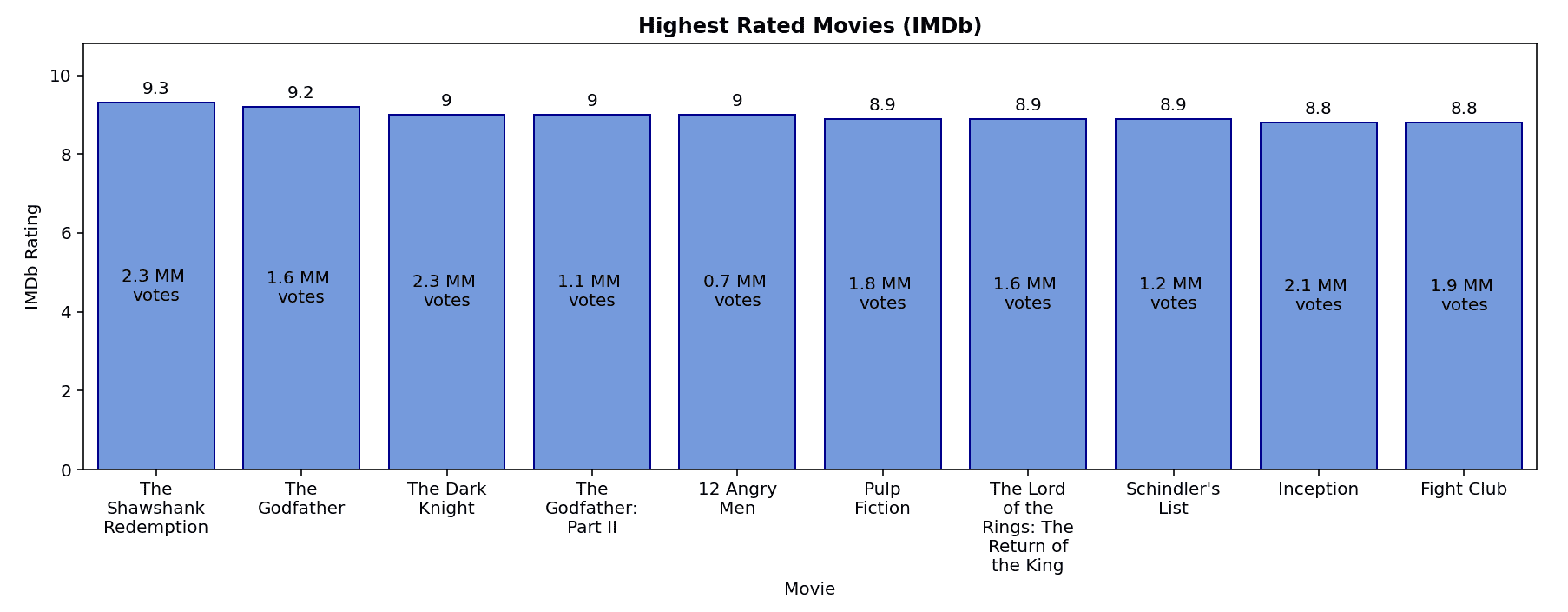
The bar chart above gives us the top 10 movies based on the highest IMBb ratings in our dataset, with the movies with the highest rating to the left and the lowest rating to the right. In case of a tie, the (non-rounded) number of votes will be the tie-breaker and determine the order of appearance. For your convenience, the number of votes (rounded per million votes) are shown on the bars. The accompanying table below the bar chart gives us additional information regarding the movies in the top 10.
• When we look at the bar chart, we see that the movie The Shawshank Redemption occupies first place in the top 10 (and therefore the entire dataset).
• Amazingly, given its IMDb rating of 9.3, it not only stands out by being the most highly IMDb rated movie, with an accumulated 2343110 votes it also boasts the highest amount of user votes out of all the movies in this top 10.
• However, with a Metascore of 80 out of 100, the movie does seem to lag in Metascore. This indicates that it wasn't as critically acclaimed as one would expect.
• Seeing as it has earned a gross revenue of USD 28.3 million, it also very much lacks in gross revenue compared to other movies in this top 10, despite some these movies having been released in the same year or earlier.
◦ For example, the movie Pulp Fiction was also released in 1994, yet it has accumulated a gross revenue of USD 107.9 million.
Other interesting observations:
• Both The Godfather and The Godfather: Part II have made it into the top 10, which is a very impressive accomplishment.
• The Godfather is the only movie in this top 10 which has earned a perfect 100 out of 100 Metascore.
• The Godfather: Part II is not the only sequel in this top 10, as The Dark Knight is also a sequel. It is the second installment in The Dark Knight trilogy. The Lord of the Rings: The Return of the King is a threequel, being the third installment of The Lord of the Rings trilogy.
• Out of all the movies in this top 10, with a gross revenue of USD 4.4 million, the movie 12 Angry Men has the lowest gross revenue by far. It being an older movie very likely plays a big part in this.
• Inception has earned the third highest gross revenue (USD 292.6 million) out of all 10 movies in this list, but with a Metascore of 74 it has earned the second-lowest Metascore.
Below, we will take a look at the top 10 highest Metascore ratings in our dataset and see how it differs from our IMDb rating top 10.
Highest Rated Movies Based On Metascore Rating
Below, we will take a look at the top 10 highest Metascore ratings in our dataset and see how it differs from our IMDb rating top 10:
| | Movie | Metascore | IMDb Rating | No of Votes | Gross in MM | Release Year |
|---|---|---|---|---|---|---|
| 1 | The Godfather | 100 | 9.2 | 1620367 | 135 | 1972 |
| 2 | Casablanca | 100 | 8.5 | 522093 | 1 | 1942 |
| 3 | Rear Window | 100 | 8.4 | 444074 | 36.8 | 1954 |
| 4 | Lawrence of Arabia | 100 | 8.3 | 268085 | 44.8 | 1962 |
| 5 | Vertigo | 100 | 8.3 | 364368 | 3.2 | 1958 |
| 6 | Citizen Kane | 100 | 8.3 | 403351 | 1.6 | 1941 |
| 7 | Trois couleurs: Rouge | 100 | 8.1 | 90729 | 4 | 1994 |
| 8 | Fanny och Alexander | 100 | 8.1 | 57784 | 5 | 1982 |
| 9 | Il conformista | 100 | 8 | 27067 | 0.5 | 1970 |
| 10 | Boyhood | 100 | 7.9 | 335533 | 25.4 | 2014 |
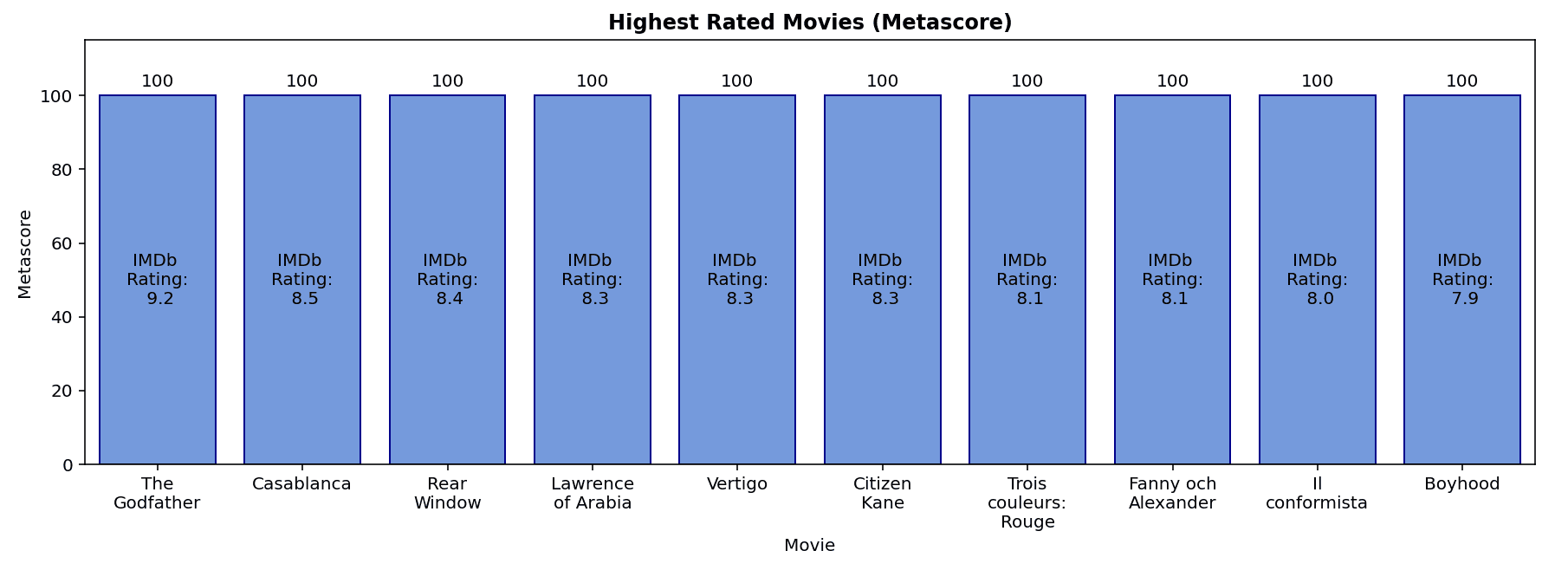
The bar chart and table above show us the top 10 movies based on the their Metascores. A quick glance reveals that all of the movies in this top 10 have a perfect Metascore of 100 out of 100. (Out of the 1000 movies in our dataset, 12 movies have managed to achieve a Metascore of 100.) Seeing as all of the movies are tied based on their Metascores, their respective IMDb ratings and their movie titles (respectively) will be the tie-breakers to determine the order of appearance.
• All movies in this list have been release before the year 2000, save for one: Boyhood, which was released in 2014.
• The number of votes vary wildly in this top 10, with 27067 votes for the movie Il conformista being the lowest and 1620367 votes for The Godfather being the highest. Their gross revenue are the lowest and highest of the top 10 as well, being USD 0.5 million and USD 135.0 million respectively.
• Three movies in this top 10 have not accumulated more than 100k votes: Trois couleurs: Rouge, Fanny och Alexander and the aforementioned Il conformista.
• The Godfather is the only movie in this top 10 which has accumulated more than a million votes.
• Although Casablanca has earned the second lowest gross revenue (USD 1.0 million) of this top 10, it has still earned a respectable 522093 number of votes on IMDb, which is the third highest of this top 10.
When we compare the top 10 movies based on IMDb rating to the top 10 movies based on Metascore, the following points stand out:
• Out of the top 10 movies with the highest IMDb ratings, only one movie seems to have made it into the top 10 movies with the highest Metascores: The Godfather.
• The gross revenues of the movies in the Metascore top 10 seem to be quite a bit lower compared to those in the IMDb ratings top 10, with the average gross revenue in the Metascore top 10 being USD 25.73 million per movie, compared to USD 167.21 million per movie in the IMDb top 10.
• Overall, the movies in the Metascore top 10 seem to be quite a bit older than those in the IMDb top 10. The average release year of the Metascore top 10 is 1969, with a median year of 1966. The IMDb top 10, on the other hand, has an average release year of 1990, with a median year of 1994.
• There also seems to be a substantial difference in the average amount of votes per movie between both top 10s. The Metascore top 10 averages 413345 votes per movie, while the IMDb top 10 has an average of 1669073 votes per movie.
• Although the average revenue, release year, and number of votes per movie are all lower in the Metascore top 10, aside from the Gross - No of Votes column pairing, the correlation coefficients between these columns aren't substantial:
◦ Release Year - Gross: 0.24
◦ Release Year - No of Votes: 0.2
◦ Gross - No of Votes: 0.56
Note: the Metascore top 10 bar chart and accompanying table above have been corrected for missing values in the Metascore and Gross in MM columns. This caused the movie Sweet Smell of Success to be replaced by the movie Boyhood. The former movie has a Metascore of 100, an IMDb Rating of 8.0, 28137 No of Votes, and a Release Year of 1957.
Metascores of the highest IMDb rated movies
Another insightful way to show the differences between the IMDb and Metascores rating systems is through showing the Metascores of the top 10 highest IMDb rated movies. The bar chart below shows us the same top 10 movies based on their IMDb ratings, which are shown on the bars. This time, however, the height of the bars is based on their respective Metascores, which are shown as values above the bars. Although we know Metascore is a weighted average score based on the scores of certain movie critics and uses a 0 to 100 scale, it might still feel a little nebulous. For instance, what is considered a reasonably good Metascore rating?

| | Movie | IMDb Rating | Metascore | Metascore Breakdown | Metascore Meaning |
|---|---|---|---|---|---|
| 1 | The Shawshank Redemption | 9.3 | 80 | 60-80 points | Generally Favorable Reviews |
| 2 | The Godfather | 9.2 | 100 | 81-100 points | Universal Acclaim |
| 3 | The Dark Knight | 9 | 84 | 81-100 points | Universal Acclaim |
| 4 | The Godfather: Part II | 9 | 90 | 81-100 points | Universal Acclaim |
| 5 | 12 Angry Men | 9 | 96 | 81-100 points | Universal Acclaim |
| 6 | Pulp Fiction | 8.9 | 94 | 81-100 points | Universal Acclaim |
| 7 | The Lord of the Rings: The Return of the King | 8.9 | 94 | 81-100 points | Universal Acclaim |
| 8 | Schindler's List | 8.9 | 94 | 81-100 points | Universal Acclaim |
| 9 | Inception | 8.8 | 74 | 60-80 points | Generally Favorable Reviews |
| 10 | Fight Club | 8.8 | 66 | 60-80 points | Generally Favorable Reviews |
To clear up the confusion a bit more, we can categorize Metascores according to the scorecard shown on their help center page. This lets us create the table above. Based on their respective Metascores, each movie falls into a certain category, shown in the column Metascore Breakdown. For example, the movie The Dark Knight has a Metascore of 84, which puts it in the category 81-100 points. As we can see in the Metascore Meaning column, it means that the movie has earned Universal Acclaim. This categorization gives us the following insights:
• As we know, the movie The Shawshank Redemption has received the highest IMDb rating in the entire dataset. Surprisingly, it has 'only' received a Metascore of 80 out of 100. This has cut it out of the 81-100 points Metascore category by 1 point, which is the highest Metascore category available. It now shares the same Metascore category as the two lowest Metascore rated movies in this top 10, which are the movies Inception and Fight Club.
• Like we previously saw in the top 10 highest IMDb rated movies, The Godfather is the only movie in this top 10 with a perfect 100 out of 100 Metascore.
• Aside from the highest IMDb rated and the two lowest IMDb rated movies, The Dark Knight, which occupies the 3rd place in this top 10, is the only movie which dips below 90 Metascore wise. All other movies score in the 90s.
Which directors and movie stars occur most in the dataset?
Being part of the top 1000 highest IMDb ranked movies is an incredible accomplishment, as every director in our dataset has influenced cinematic history through their work. Although quantity might not be an accurate way to measure a person's influence on said history because it doesn't paint the whole picture, it is still of value to see which directors and actors have graced our dataset with the most occurrences. Knowing the prominent figures within our dataset and to what extent they have proven to consistently deliver high-quality movies helps us to identify and understand trends. It sets benchmarks for quality and reveals patterns.
Firstly, we will first take a look at the most occurring directors in our dataset. A director is one of the, if not the most influential person in the process of creating a movie. Directors are the creative visionaries tasked with translating a screenplay into a movie, all the while making important decisions on the style, tone, pacing and overall artistic vision of the movie.
From there, we will move on and take a look at the most occurring occuring movie stars in our dataset. Out of all the people involved in creating a movie, movie stars are obviously the most recognizable to us. Even if you are not a movie buff, you will most likely recognize at least one name in this list. It is to no one's surprise that they are absolutely crucial in bringing characters (and stories) to life.
Top 10 directors based on movie count
| | Director | No of Movies | AVG IMDb Rating | AVG No of Votes | Min Release Year | Max Release Year | Diff. Min/Max Years | AVG Release Year | Median Release Year |
|---|---|---|---|---|---|---|---|---|---|
| 1 | Alfred Hitchcock | 14 | 8 | 192613 | 1935 | 1963 | 28 | 1949 | 1950 |
| 2 | Steven Spielberg | 13 | 8 | 601320 | 1975 | 2015 | 40 | 1990 | 1989 |
| 3 | Hayao Miyazaki | 11 | 8 | 213520 | 1979 | 2013 | 34 | 1994 | 1992 |
| 4 | Martin Scorsese | 10 | 8.2 | 651353 | 1976 | 2019 | 43 | 1995 | 1992 |
| 5 | Akira Kurosawa | 10 | 8.2 | 94160 | 1950 | 1985 | 35 | 1962 | 1960 |
| 6 | Stanley Kubrick | 9 | 8.2 | 435473 | 1956 | 1987 | 31 | 1968 | 1968 |
| 7 | Billy Wilder | 9 | 8.1 | 115323 | 1944 | 1960 | 16 | 1952 | 1953 |
| 8 | Woody Allen | 9 | 7.8 | 135834 | 1975 | 2011 | 36 | 1987 | 1985 |
| 9 | Christopher Nolan | 8 | 8.5 | 1447293 | 2000 | 2017 | 17 | 2009 | 2009 |
| 10 | Quentin Tarantino | 8 | 8.2 | 1015401 | 1992 | 2019 | 27 | 2006 | 2006 |
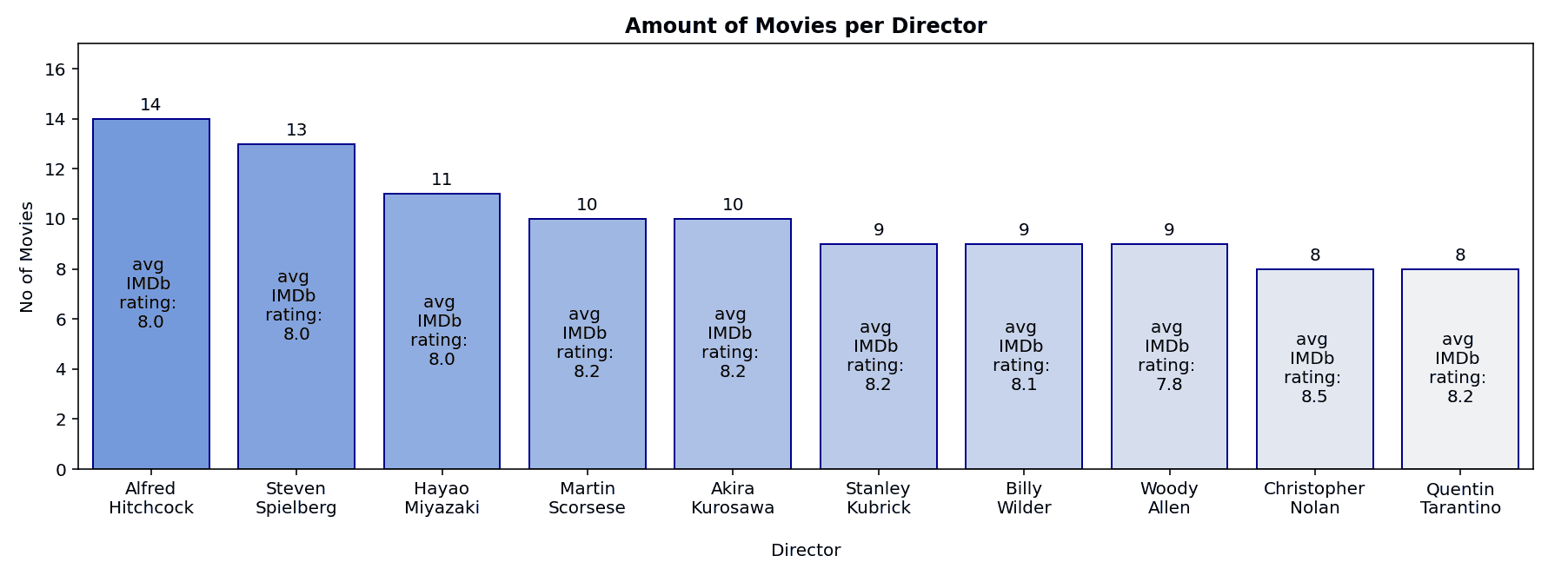
On the bar chart above we see the top 10 movie directors based on how many of their movies occur in this dataset. The accompanying table below it gives us additional information and context on their careers. Combined, they gives us valuable insights into the great work which has solidified their place in cinematic history. In case directors have an equal amount of movies present in the dataset, we will use the average IMDb rating of their movies and their average number of votes per movie (respectively) as a tie-breakers to determine their position in the top 10. The most important takes are as follows:
• The top spot is taken by Alfred Hitchcock with 14 movies in this dataset, with an average IMDb rating of 8.0.
◦ Although many of us have probably heard his name, not everyone has seen one (or more) of his movies. This is most likely due to the time period in which he was active as a director. His earliest release year in this data set is 1935, with the average release of his movies being 1949, the median release year being 1950, and a maximum release year of 1963, all of which are the lowest in the entire top 10.
• As the runner-up, Steven Spielberg is right on his heels with 13 movies present in our dataset, with an average IMDb rating of 8.0
◦ The name Steven Spielberg will most likely ring a bell, as he is one the most well known directors alive. Based on his earliest and most recent movie releases, his career has spanned 40 years (and counting), which is the second longest out of all the directors in this top 10. First place belongs to director Martin Scorsese with 43 years. Amazingly, at the moment of writing, both of them are still directing movies.
◦ Obviously, the difference between a director's earliest and most recent movie release year doesn't fully equate career span, because not only are some directors still active, it also doesn't include movies which have not made it into this top 1000. But, at the very least it gives us an idea of how long their career has spanned at minimum.
• Hayao Miyazaki makes for an interesting third place, as all of his movies in our dataset (as well as his entire filmography) are animated movies.
• The director Akira Kurosawa averages 94160 amount of votes per movie, which is the lowest of the entire top 10 and the only average amount of votes not breaking the 100k boundary.
• Woody Allen is the only director whose average IMDb rating per movie dips into the 7s; every other director's average IMDb rating is in the 8s.
• Only two directors have an average amount of votes per movie in the millions: Christopher Nolan and Quentin Tarantino. With respective IMDb ratings of 8.5 and 8.2, they have the highest and (shared) second highest IMDb ratings of all the directors in this top 10.
Top 10 movie stars based on movie count
| | Movie Star | No of Movies | AVG IMDb Rating | AVG No of Votes | Min Release Year | Max Release Year | Diff. Min/Max Years | AVG Release Year | Median Release Year |
|---|---|---|---|---|---|---|---|---|---|
| 1 | Robert De Niro | 17 | 8.1 | 458073 | 1974 | 2019 | 45 | 1991 | 1990 |
| 2 | Tom Hanks | 14 | 8 | 669583 | 1993 | 2019 | 26 | 2002 | 2000 |
| 3 | Al Pacino | 13 | 8.1 | 469109 | 1972 | 2019 | 47 | 1989 | 1992 |
| 4 | Brad Pitt | 12 | 8 | 762061 | 1995 | 2019 | 24 | 2005 | 2004 |
| 5 | Clint Eastwood | 12 | 8 | 279404 | 1964 | 2008 | 44 | 1980 | 1974 |
| 6 | Leonardo DiCaprio | 11 | 8.1 | 980200 | 1993 | 2019 | 26 | 2008 | 2010 |
| 7 | Christian Bale | 11 | 8 | 778720 | 1987 | 2019 | 32 | 2007 | 2007 |
| 8 | Matt Damon | 11 | 8 | 621853 | 1997 | 2019 | 22 | 2006 | 2006 |
| 9 | James Stewart | 10 | 8.1 | 172429 | 1939 | 1962 | 23 | 1950 | 1949 |
| 10 | Michael Caine | 9 | 8.1 | 673832 | 1972 | 2014 | 42 | 1996 | 2005 |
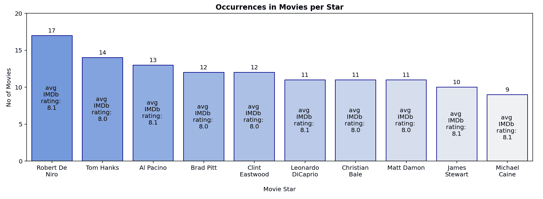
On the bar chart above you will see the movie stars with the most amount of occurrences in our dataset, irregardless of the actor category they belong to ('star1', 'star2', 'star3' or 'star4'). The accompanying table beneath the bar chart gives us more information (in aggregate) on their release years and number of votes. Similar to the movie directors bar chart above, we will use the average IMDb rating of their movies and their average number of votes per movie (respectively) as a tie-breakers to determine their position in the top 10. The most interesting observations are as follows:
• As can be seen on the chart, the movie star with the most occurrences in our list is Robert De Niro, with 17 movie occurrences with an average IMDb rating of 8.1.
◦ Based on this top 10, with an earliest release year of 1974 and a most recent release year of 2019, Robert De Niro has had the second longest movie career span: 45 years (and counting). First place goes to the (still active) Al Pacino with 47 years.
◦ The same caveat with regards to career span is applicable here: the difference between an actor's earliest and most recent movie release year doesn't fully equate career span. However, it does give us an idea of how long their career has spanned at minimum.
• The runner up of having the most movies in this dataset is Tom Hanks, with 14 movies under his belt and an average IMDb rating of 8.0.
◦ Compared to Robert De Niro, Tom Hanks only has 26 years of difference between his first and most recent movies in this dataset, compared to Robert De Niro's 45 years.
• With an average of 980200 votes per movie, Leonardo DiCaprio has the highest average number of votes in this top 10. To compare, the runner up is Christian Bale with an average of 778720 voters per movie.
• James Stewart has the lowest minimum, maximum, average and median release years out of all the movie stars in this top 10, as well as the lowest average amount of votes per movie.
Comparing the Directors and Movie Stars Top 10s
When we compare the directors top 10 with the movie star top 10, we can make the following observations:
• In contrast to certain directors (Christopher Nolan and Quentin Tarantino), no movie star in the top 10 has broken a million average amount of votes per movie. Leonardo DiCaprio came close, with an average of 980200 votes per movie. Interestingly, the average amount of votes for directors (490229 votes) is lower than for movie stars (586526 votes).
• Aside from Clint Eastwood and the late James Stewart, the most recent release years of most movie stars are fairly recent. At the moment of writing, aside from the these two exceptions, all of the movie stars in this top 10 are either still acting or have done so up until fairly recently. (Clint Eastwood is currently still active as a movie director. He has announced his upcoming movie to be his last.) In comparison, many directors' most recent work in this dataset is a bit less recent, as some of them have since past away.
• Compared to the directors top 10, there's not a whole lot of variety to be found in the AVG IMDb Rating column in the movie stars top 10. Movie stars either have an average IMDb rating of 8.0 or 8.1. This is different in the directors top 10, where the average IMDb rating ranges from 7.8 to 8.5.
◦ Only one actor (Michael Caine) in our movie stars top 10 hasn't reached double digits in movie count, while half of the directors haven't done so in the directors top 10.
Closing Thoughts
We have now reached the end of this explorative data analysis on the top 1000 IMDb movies dataset. Among other things, together, we have navigated the intricacies of rating distribution, genre pairings and the most occuring names in our dataset. We have traversed a trip through time, filled with names which will forever be part of cinematic history. As we wrap up this report, it’s clear that the world of cinema is as diverse and dynamic as the audience it serves. As we have seen, it is ever evolving. Whether you’re a casual viewer or a dedicated cinephile, I hope you have found this EDA to be insightful and at least somewhat entertaining.
If you have any questions or remarks with regard to this EDA (or anything else), please don't hesitate to contact me through the contact form on this website.